F/I-SAPT: Functional Group and/or Intramolecular SAPT
Code author: Robert M. Parrish
Section author: Robert M. Parrish
Module: Keywords, PSI Variables, FISAPT
The FISAPT module provides two extensions to standard SAPT theory to allow for (1) an effective two-body partition of the various SAPT terms to localized chemical functional groups (F-SAPT) and (2) a means to compute the SAPT interaction between two moieties within the embedding field of a third body (I-SAPT). F-SAPT is designed to provide additional insight into the chemical origins of a noncovalent interaction, while I-SAPT allows for one to perform a SAPT analysis for intramolecular interactions. F-SAPT and I-SAPT can be deployed together in this module, yielding “F/I-SAPT.” All F/I-SAPT computations in PSI4 use density-fitted SAPT0 as the underlying SAPT methodology. Interested users should consult the manual page for Ed Hohenstein’s SAPT0 code and the SAPT literature to understand the specifics of SAPT0 before beginning with F/I-SAPT0.
F-SAPT is detailed over two papers: [Parrish:2014:044115] on our much-earlier “atomic” SAPT (A-SAPT) and [Parrish:2014:4417] on the finished “functional group” SAPT (F-SAPT). An additional paper describes how to use F-SAPT to analyze differences under functional group substitutions [Parrish:2014:17386]. I-SAPT is explained in [Parrish:2015:051103]. There is also a reasonably-detailed review of the aims of A/F/I-SAPT and the existing state-of-the-art in the field in the introduction chapter on partitioned SAPT methods in Parrish’s thesis.
The scripts discussed below are located in psi4/psi4/share/psi4/fsapt.
F-SAPT: A Representative Example
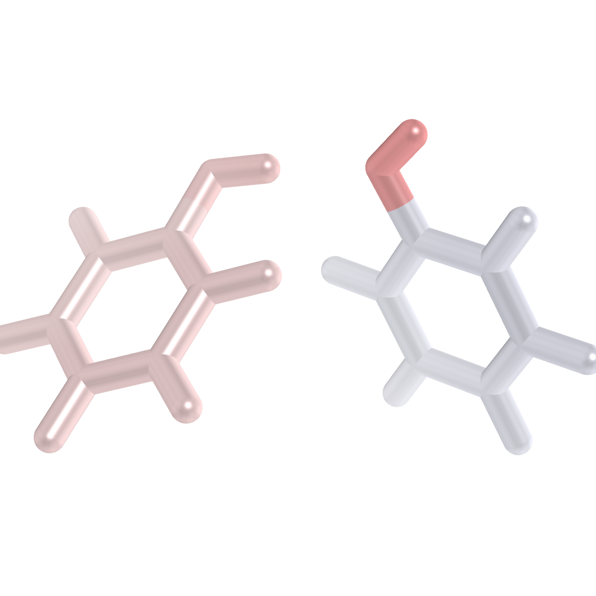
Below, we show an example of using F-SAPT0/jun-cc-pVDZ to analyze the distribution of the intermolecular interaction energy components between the various hydroxyl and phenyl moieties of the phenol dimer. This example is explicitly included in fsapt1. A video lecture explaining this example is available F-SAPT#1, while an additional video describing how to plot the order-1 F-SAPT analysis with PyMol and perform a “difference F-SAPT” analysis is available F-SAPT#2:
memory 1 GB

molecule mol {
0 1
O    -1.3885044    1.9298523   -0.4431206
H    -0.5238121    1.9646519   -0.0064609
C    -2.0071056    0.7638459   -0.1083509
C    -1.4630807   -0.1519120    0.7949930
C    -2.1475789   -1.3295094    1.0883677
C    -3.3743208   -1.6031427    0.4895864
C    -3.9143727   -0.6838545   -0.4091028
C    -3.2370496    0.4929609   -0.7096126
H    -0.5106510    0.0566569    1.2642563
H    -1.7151135   -2.0321452    1.7878417
H    -3.9024664   -2.5173865    0.7197947
H    -4.8670730   -0.8822939   -0.8811319
H    -3.6431662    1.2134345   -1.4057590
--
0 1
O     1.3531168    1.9382724    0.4723133
H     1.7842846    2.3487495    1.2297110
C     2.0369747    0.7865043    0.1495491
C     1.5904026    0.0696860   -0.9574153
C     2.2417367   -1.1069765   -1.3128110
C     3.3315674   -1.5665603   -0.5748636
C     3.7696838   -0.8396901    0.5286439
C     3.1224836    0.3383498    0.8960491
H     0.7445512    0.4367983   -1.5218583
H     1.8921463   -1.6649726   -2.1701843
H     3.8330227   -2.4811537   -0.8566666
H     4.6137632   -1.1850101    1.1092635
H     3.4598854    0.9030376    1.7569489
symmetry c1
no_reorient
no_com
}

set {
basis         jun-cc-pvdz
scf_type df
guess sad
freeze_core true
}

energy('fisapt0')
This file runs a DF-HF computation on the full dimer using PSI4‘s existing
SCF code. The monomer SCF computations are performed inside the FISAPT module,
following which a complete DF-SAPT0 computation is performed. Additional bits of
analysis are performed to generate the order-2 partition of the SAPT terms to
the level of nuclei and localized occupied orbitals – this generally does not
incur much additional overhead beyond a standard SAPT0 computations. The
nuclear/orbital partition data is written to the folder fsapt/ in the same
directory as the input file (this can be changed by FISAPT_FSAPT_FILEPATH).
One obtains the desired F-SAPT partition by post-processing the data in
fsapt/. Within this dir, the user is expected to provide the ASCII files
fA.dat and fB.dat, which describe the assignment of atoms to chemical
functional groups using 1-based ordering. E.g., for the problem at hand,
fA.dat contains:
OH 1 2
PH 3 4 5 6 7 8 9 10 11 12 13
while fB.dat contains:
OH 14 15
PH 16 17 18 19 20 21 22 23 24 25 26
At this point, the user should run the fsapt.py post-processing script in
the fsapt directory as:
>>> fsapt.py
This will generate, among other files, the desired functional-group partition in
fsapt.dat. For our problem, the bottom of this file contains the finished
partition:
Frag1     Frag2          Elst      Exch     IndAB     IndBA      Disp     Total
OH        OH           -8.425     6.216    -0.583    -1.512    -1.249    -5.553
OH        PH            1.392     0.716     0.222    -0.348    -0.792     1.189
PH        OH           -2.742     0.749    -0.147    -0.227    -0.674    -3.040
PH        PH            0.680     2.187     0.007    -0.208    -2.400     0.266
OH        All          -7.033     6.931    -0.362    -1.860    -2.040    -4.364
PH        All          -2.062     2.936    -0.140    -0.435    -3.074    -2.774
All       OH          -11.167     6.965    -0.730    -1.739    -1.923    -8.594
All       PH            2.072     2.903     0.229    -0.556    -3.191     1.456
All       All          -9.095     9.867    -0.501    -2.295    -5.114    -7.138
Note that the assignment of linking sigma bond contributions is a small point of
ambiguity in F-SAPT. The fsapt.dat file presents the “links-by-charge”
assignment at the top and the “links by 50-50” assignment at the bottom. We
generally prefer the latter, but both generally give qualitatively identical
energetic partitions.
Users should check the files fragA.dat and fragB.dat to ensure that
there is not too much charge delocalization from one fragment to another. This
is presented in the “Orbital Check” section in these files – a value larger than
0.1 docc is an indication that the picture of localizable functional groups may
be breaking down. We also strongly discourage the cutting of double,
triple, or aromatic bonding motifs when partitioning the molecule into fragments
– cuts across only simple sigma bonds are encouraged.
Caution
November 2022, previous to QCEngine v0.26.0 and Psi4
v1.7.0, there was a scaling inconsistency in the pairwise analysis
such that 2-BODY PAIRWISE DISPERSION CORRECTION ANALYSIS
was doubled when generated from dftd3 compared to the output from other
programs (s-dftd3 and dftd4). This shows up in the QCVariable and in the
Empirical_Disp.dat file written during energy("fisapt0-d3") (all
-D3 variants). Fortunately, the fsapt.py script compensated
for dftd3 (by far the most used program for this task). Users of the
pairwise analysis should take care to use the new QCEngine
AND fsapt.py script distributed with NEW Psi4. fisapt0-d4 run
with previous Psi4/fsapt.py will be wrong. fisapt0-d3 run with previous
Psi4/fsapt.py but new QCEngine will be wrong. If you’ve got legacy
calculations, it is extremely easy to check or reanalyze them to
salvage them, so please contact the developers with the circumstances
for guidance.
Python F-SAPT Analysis
Now F-SAPT post-processing can be performed within python without the need to
use output files and fsapt.py. The following code snippet performs the same
analysis as above, but directly within python:
import psi4


mol = psi4.geometry(
    """0 1
0 1
O    -1.3885044    1.9298523   -0.4431206
H    -0.5238121    1.9646519   -0.0064609
C    -2.0071056    0.7638459   -0.1083509
C    -1.4630807   -0.1519120    0.7949930
C    -2.1475789   -1.3295094    1.0883677
C    -3.3743208   -1.6031427    0.4895864
C    -3.9143727   -0.6838545   -0.4091028
C    -3.2370496    0.4929609   -0.7096126
H    -0.5106510    0.0566569    1.2642563
H    -1.7151135   -2.0321452    1.7878417
H    -3.9024664   -2.5173865    0.7197947
H    -4.8670730   -0.8822939   -0.8811319
H    -3.6431662    1.2134345   -1.4057590
--
0 1
O     1.3531168    1.9382724    0.4723133
H     1.7842846    2.3487495    1.2297110
C     2.0369747    0.7865043    0.1495491
C     1.5904026    0.0696860   -0.9574153
C     2.2417367   -1.1069765   -1.3128110
C     3.3315674   -1.5665603   -0.5748636
C     3.7696838   -0.8396901    0.5286439
C     3.1224836    0.3383498    0.8960491
H     0.7445512    0.4367983   -1.5218583
H     1.8921463   -1.6649726   -2.1701843
H     3.8330227   -2.4811537   -0.8566666
H     4.6137632   -1.1850101    1.1092635
H     3.4598854    0.9030376    1.7569489
symmetry c1
no_reorient
no_com
"""
)
psi4.set_options(
    {
        "basis": "jun-cc-pvdz",
        "scf_type": "df",
        "guess": "sad",
        "freeze_core": "true",
        "FISAPT_FSAPT_FILEPATH": "none",
    }
)
plan = psi4.energy("fisapt0", return_plan=True, molecule=mol)
atomic_result = psi4.schema_wrapper.run_qcschema(
    plan.plan(),
    clean=True,
    postclean=True,
)
fEnergies = psi4.fsapt_analysis(
    source=atomic_result, # AtomicResult from QCSchema
    # NOTE: 1-indexed for fragments_a and fragments_b
    fragments_a={
        "MethylA": [1, 2, 3, 4, 5],
    },
    fragments_b={
        "MethylB": [6, 7, 8, 9, 10],
    },
)
# Or you can use energy calls without QCSchema with this example below
# using the same molecule and options as above.
e, wfn = psi4.energy("fisapt0", return_wfn=True)
data = psi4.fsapt_analysis(
    source=wfn, # through wavefunction object
    # NOTE: 1-indexed for fragments_a and fragments_b
    fragments_a={
        "MethylA": [1, 2, 3, 4, 5],
    },
    fragments_b={
        "MethylB": [6, 7, 8, 9, 10],
    },
)
Additionally, if you have F-SAPT data from saving results to
FISAPT_FSAPT_FILEPATH, you can use psi4.fsapt_analysis to read in the data
and perform the analysis without needing to run fsapt.py by specifying the
filepath as in:
import psi4


psi4.fsapt_analysis(
    fragments_a={
        "MethylA": [1, 2, 3, 4, 5],
    },
    fragments_b={
        "MethylB": [6, 7, 8, 9, 10],
    },
    source="./fsapt",
)
Order-1 Visualization with PyMol
The fsapt.py script above also generates a number of order-1 .pdb files
that can be used to get a quick qualitative picture of the F-SAPT partition. The
preferred way to do this is to use PyMol to make plots of the molecular geometry
with the atoms colored according to their order-1 F-SAPT contributions. We have
a set of template .pymol scripts to help with this process. These can be
obtained by running:
>>> copy_pymol.py
and then in PyMol:
>>> @run.pymol
This last command runs all of the individual .pymol files (e.g.,
Elst.pymol), which in turn load in the molecule and order-1 analysis
(contained in the .pdb file), set up the visualization, and render a
.png image of the scene. Generally the view orientation and some specific
details of the .pymol files require some small tweaks to permit
publication-quality renderings.
Difference F-SAPT Analysis
For those interested in taking the differences between two F-SAPT partitions
(e.g., to see how a substituent modulates a noncovalent interaction), we have
the fsapt-diff.py script to help with this. This is invoked as:
>>> fsapt-diff.py source-fsapt-dir1 source-fsapt-dir2 target-diff-fsapt-dir
Where the use has already performed fsapt.py analysis using the same
functional group names in source-fsapt-dir-1 and source-fsapt-dir-2. The
difference F-SAPT partition entries are computed as \(E^{\Delta} = E^{1} -
E^{2}\), and the geometries for order-1 .pdb visualization files are taken
from system 1.
I-SAPT: A Representative Example
Note
Molecule fragments must each have physically plausible multiplicity
(unlike the singlet OH fragments in the bad_mol example below), and the
overall molecule needs to be a singlet. For situations like this, you’ll need
to specify the overall charge and multiplicity and set physical multiplicities
for each fragment, either through the usual string syntax (good_mol below)
or through psi4.core.Molecule.from_arrays(). Examples are in
isapt1 and isapt-charged.
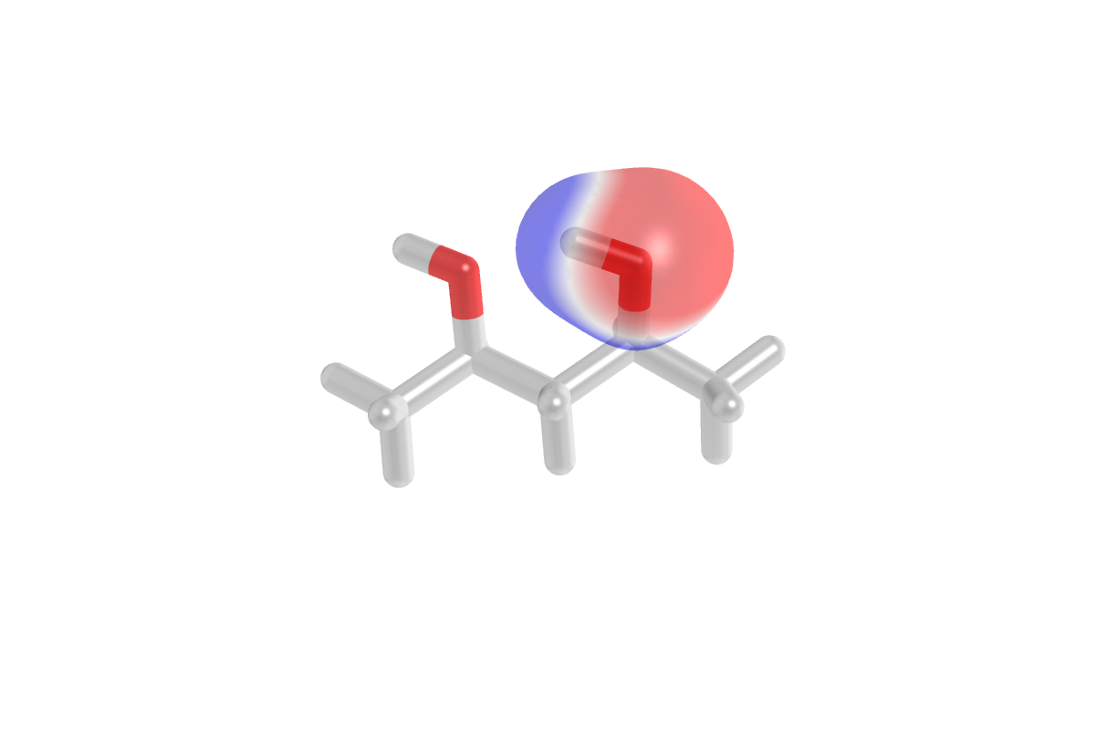
Below, we show an example of using I-SAPT0/jun-cc-pVDZ to analyze the interaction between the two phenol groups in a 2,4-pentanediol molecule. This example is explicitly included in isapt1. A video lecture explaining this example is available I-SAPT#1, while an additional video describing how to plot the density and ESP fields from the I-SAPT embedding procedure is available I-SAPT#2:
memory 1 GB

# won't work with all singlets
molecule bad_mol {
0 1
O          0.39987        2.94222       -0.26535
H          0.05893        2.05436       -0.50962
--
0 1
O          0.48122        0.30277       -0.77763
H          0.26106       -0.50005       -1.28451
--
0 1
C          2.33048       -1.00269        0.03771
C          1.89725        0.31533       -0.59009
C          2.28232        1.50669        0.29709
C          1.82204        2.84608       -0.29432
C          2.37905        4.02099        0.49639
H          3.41246       -1.03030        0.19825
H          2.05362       -1.84372       -0.60709
H          1.82714       -1.16382        0.99734
H          2.36243        0.42333       -1.57636
H          3.36962        1.51414        0.43813
H          1.81251        1.38060        1.28140
H          2.14344        2.92967       -1.33843
H          3.47320        4.02400        0.48819
H          2.03535        3.99216        1.53635
H          2.02481        4.96785        0.07455
symmetry c1
no_reorient
no_com
}

# will work with total and per-fragment charge and multiplicity
molecule good_mol {
0 1
--
0 2
O          0.39987        2.94222       -0.26535
H          0.05893        2.05436       -0.50962
--
0 2
O          0.48122        0.30277       -0.77763
H          0.26106       -0.50005       -1.28451
--
0 1
C          2.33048       -1.00269        0.03771
C          1.89725        0.31533       -0.59009
C          2.28232        1.50669        0.29709
C          1.82204        2.84608       -0.29432
C          2.37905        4.02099        0.49639
H          3.41246       -1.03030        0.19825
H          2.05362       -1.84372       -0.60709
H          1.82714       -1.16382        0.99734
H          2.36243        0.42333       -1.57636
H          3.36962        1.51414        0.43813
H          1.81251        1.38060        1.28140
H          2.14344        2.92967       -1.33843
H          3.47320        4.02400        0.48819
H          2.03535        3.99216        1.53635
H          2.02481        4.96785        0.07455
symmetry c1
no_reorient
no_com
}

# => Standard Options <= #

set {
basis jun-cc-pvdz
scf_type df
guess sad
freeze_core true
fisapt_do_plot true  # For extra analysis
}

energy('fisapt0')
This is essentially the same input as for F-SAPT, except that the molecular system is now divided into three moieties – subsystems A and B whose intramolecular interaction we wish to compute, and a linking unit C. This file runs a DF-HF computation on the full system using PSI4‘s existing SCF code. At the start of the FISAPT code, the occupied orbitals are localized and divided by charge considerations into A, B, C, and link sets. By default, linking sigma bonds are assigned to C (this can be changed by the FISAPT_LINK_ASSIGNMENT options). Then, non-interacting Hartree–Fock solutions for A and B are optimized in the embedding field of the linking moiety C. At this point, A and B are not interacting with each other, but have any potential covalent links or other interactions with C built in by the embedding. A standard F-SAPT0 computation is then performed between A and B, yielding the I-SAPT interaction energy. Any F-SAPT considerations are also possible when I-SAPT is performed – F and I are completely direct-product-separable considerations.
Cube File Visualization with PyMol
Setting FISAPT_DO_PLOT true above generates a set of .cube files
containing the densities and ESPs of the various subsystems in the I-SAPT
embedding procedure. These can be used to gain a detailed understanding of the
intermolecular partition and the polarization between non-interacting and
Hartree–Fock-interacting moieties. We have developed a set of template
.pymol scripts to help with this process. These can be obtained by running:
>>> copy_pymol2.py
and then in PyMol:
>>> @run.pymol
This last command runs all of the individual .pymol files (e.g.,
DA.pymol), which in turn load in the molecule and cube file data
(contained in the .cube file), set up the visualization, and render a
.png image of the scene. Generally the view orientation and some specific
details of the .pymol files require some small tweaks to permit
publication-quality renderings.
Adding Point Charges to F/I-SAPT Computations
Point charges can be added to the interacting subsystems A and B as well
as to the linking fragment C. Briefly, the interaction between the point charges in A(B)
and fragment B(A) enters the SAPT0 interaction energy. It explicitly affects the electrostatics
and induction components, and implicitly affects other SAPT0 components by polarizing the orbitals.
If point charges are present in both subsystems A and B, an additional charge-charge interaction
term is also added to the electrostatic energy. When point charges are assigned to subsystem C, the point
charges in C only polarize the orbitals in both fragment A and B. However, the presence of charges in C does not
directly contribute to the SAPT0 interaction energy.
Examples fsapt-ext-abc and fsapt-ext-abc2 illustrate the use of point charges in F/I-SAPT procedure.
Link Orbital Partitioning in I-SAPT
The assignment of the A-C and B-C linking electron pairs is controlled by the FISAPT_LINK_ASSIGNMENT
keyword. The default setting fisapt_link_assignment c assigns the entire pair to the linker C together with
a +1 nuclear charge from the connecting atoms of A/B to preserve the electrical neutrality of each fragment.
However, as already noticed in [Parrish:2015:051103], such a partitioning might result in unphysical dipole
moments at the interfragment boundaries. Imagine, for example, that I-SAPT is used to examine the interaction
of two methyl groups connected by some linker fragment. When the linking bonds are assigned to C, the carbon atoms
of the methyl groups are missing electrons on one of their sp^3 hybrid orbitals and a dipole moment appears.
These dipole moments have been observed to lead, in some cases, to I-SAPT energy contributions that do not make
physical sense, for example, to a strongly repulsive electrostatic energy between two fragments connected by an
intramolecular hydrogen bond.
To overcome this issue, Luu and Patkowski proposed a reassignment of the linking electron pairs so that each fragment
(C and A/B) gets one electron [Luu:2023:356]. This electron is placed on a hybrid orbital of the connecting atom
pointing in the direction of the interfragment bond. Several schemes for determining this link hybrid were proposed
in [Luu:2023:356] and they all are implemented in PSI4. We recommend the so-called SIAO1 scheme,
fisapt_link_assignment siao1, as it has been observed to provide consistently meaningful I-SAPT terms and a
smooth basis set convergence. The SIAO1 name implies that the projection to construct the link hybrids happens in the
intrinsic atomic orbital space (as opposed to the SAO1 method where the standard atomic orbital space is used), with
one iteration of fragment orbital optimization and link orbital orthogonalization, a process that very quickly
achieves self-consistency. Altogether, the allowed values for FISAPT_LINK_ASSIGNMENT are c (default),
ab (the opposite of c where the entire linking pair is assigned to A/B), sao0, sao1, sao2,
siao0, siao1 (recommended for all I-SAPT applications), and siao2 (essentially identical to siao1 but
slightly more expensive).
Advanced I-SAPT Keywords for SAOn/SIAOn Partitionings
FISAPT_LINK_ORTHO
Orthogonalization of link orbitals for FISAPT_LINK_ASSIGNMENT=SAOx/SIAOx Link A orthogonalized to A in whole (interacting) molecule or in the (noninteracting) fragment?
Type: string
Possible Values: FRAGMENT, WHOLE, NONE
Default: FRAGMENT
FISAPT_EXCH_PARPERP
Calculate separate exchange corrections for parallel and perpendicular spin coupling of link orbitals? When false, only the averaged out exchange corrections are computed.
Type: boolean
Default: false
FISAPT_CUBE_LINKIBOS
Generate cube files for unsplit link orbitals (IBOs)?
Type: boolean
Default: false
FISAPT_CUBE_LINKIHOS
Generate cube files for split link orbitals (IHOs)?
Type: boolean
Default: false
FISAPT_CUBE_DENSMAT
Generate cube files for fragment density matrices?
Type: boolean
Default: false
Other F/I-SAPT Keywords
The input files described above cover roughly 90% of all F/I-SAPT analyses. For more delicate or involved problems, there are a large number of user options that permit the customization of the I-SAPT subsystem partition, the convergence of the IBO localization procedure, numerical thresholds, etc. We have an entire video tutorial devoted to F/I-SAPT Options . Direct source-code documentation on these options is available here.
Additional Notes
Caution
In constrast to Ed Hohenstein’s SAPT0 code, FISAPT uses the -JKFIT auxiliary basis sets for all Fock-type terms (e.g., electrostatics, exchange, induction, and core Fock matrix elements in exchange-dispersion), and the -RI auxiliary basis sets only for the dispersion term. Ed’s code uses the -RI basis sets for all SAPT terms, which can be problematic for heavy elements. As such, Ed’s SAPT0 code will yield slightly different results than FISAPT. The differences should be very minor for up to and including second-row elements, after which point one needs to use the DF_BASIS_ELST option in Ed’s code to provide an accurate result.